This notebook assumes basic knowledge about training neural networks, what a CNN is and other deep learning knowledge such as batchnorm and basic knowledge of sound represented in digital format.
To learn about the latter, you can go through this 6-part blog series that goes from the beginning explaining about the issue. (The first four posts will be sufficient for this notebook)
Imports
import randomfrom collections import Counterimport librosaimport numpy as npimport pandas as pdimport matplotlib.pyplot as pltimport seaborn as snsfrom sklearn.model_selection import train_test_splitfrom fastcore.allimport*import torchimport torch.nn as nnimport torch.nn.functional as Fimport torch.optim as optimfrom torch.utils.data import Dataset, DataLoader, random_split, WeightedRandomSamplerimport torchaudioimport torchaudio.transforms as Tfrom IPython.display import Audio, display
Introduction
Respiratory sounds are important indicators of respiratory health and respiratory disorders. The sound emitted when a person breathes is directly related to air movement, changes within lung tissue and the position of secretions within the lung. A wheezing sound, for example, is a common sign that a patient has an obstructive airway disease like asthma or chronic obstructive pulmonary disease (COPD).
These sounds can be recorded using digital stethoscopes and other recording techniques. This digital data opens up the possibility of using machine learning to automatically diagnose respiratory disorders like asthma, pneumonia and bronchiolitis, to name a few.
In this notebook, we are going to try and create a Convolutional Neural Network that can distinguish and classify different respiratory sounds and make a diagnosis. In the process, we are going to learn about how sound is represented in digital format, converting the audio files into spectrograms, which the CNN can use to learn from and a few other random things about training neural networks.
I learned a lot from other people while making this notebook and I reference all of them at the bottom.
Getting the Data
Luckily for us, two research teams in Portugal and Greece already prepared a suitable dataset that can be found on Kaggle. It includes 920 annotated recordings of varying length - 10s to 90s. These recordings were taken from 126 patients. There are a total of 5.5 hours of recordings containing 6898 respiratory cycles.
We can download the dataset using the kaggle command.
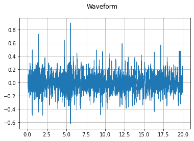
As you can see, the waveform is still a signal. A CNN expects an image-like input. So we need a way to convert the above signal to an image. A Spectrogram is a visual representation of spectrum of frequencies of a signal as it varies with time
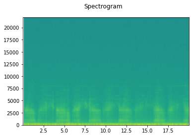
Here is a spectrogram of the example audio above:
plot_specgram(waveform, sample_rate);
/usr/local/lib/python3.7/dist-packages/matplotlib/axes/_axes.py:7592: RuntimeWarning: divide by zero encountered in log10
  Z = 10. * np.log10(spec)
As you can see, just and ordinary spectrogram won’t give our CNN much to learn from. Mel Spectrograms work better in this case. Converting a Spectrogram to a Mel spectogram is easy in PyTorch.
/usr/local/lib/python3.7/dist-packages/torchaudio/functional/functional.py:433: UserWarning: At least one mel filterbank has all zero values. The value for `n_mels` (128) may be set too high. Or, the value for `n_freqs` (513) may be set too low.
  "At least one mel filterbank has all zero values. "
This is a better visual representation than ordinary spectrograms and gives our neural network something to work with.
Finally, we can play the audio and hear the respiratory recording.
play_audio(waveform, sample_rate);
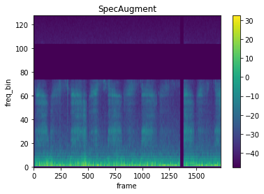
Audio Data Augmentation (SpecAugment by Google)
To make training robust in Deep Learning, we usually utilize Data Augmentation which is artificially creating new data from the data we have. This also helps with regularizing the model to curb overfitting.
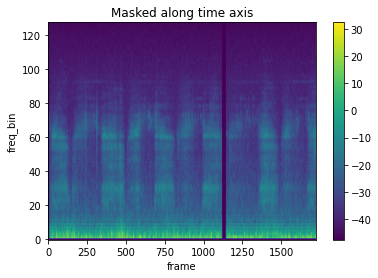
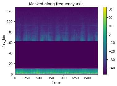
But for our data, we can’t just use the normal augmentations we use on images, like flip and rotate. Google came up with a nice augmentation specifically called SpecAugment. This involves maksing our Mel Spectograms on either the time axis (Time Masking) or along the frequency axis (Frequency Masking).
torchaudio makes this easier for us to implement the following transforms. Here are the corresponding outputs when we apply the specific masking:
Time Masking
time_masking = T.TimeMasking(time_mask_param=80)spec = time_masking(melspec)plot_spectrogram(spec[0], title="Masked along time axis")
Frequency Masking
freq_masking = T.FrequencyMasking(freq_mask_param=80)spec = freq_masking(melspec)plot_spectrogram(spec[0], title="Masked along frequency axis")
For our specific task, we are going to be utilizing both of the two transform simultaneously.
/usr/local/lib/python3.7/dist-packages/seaborn/_decorators.py:43: FutureWarning: Pass the following variable as a keyword arg: x. From version 0.12, the only valid positional argument will be `data`, and passing other arguments without an explicit keyword will result in an error or misinterpretation.
  FutureWarning
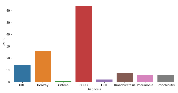
As with many medical datasets, we can already see massive imbalance in the data. This is a disadvantage since our model can just learn to predict the most common class and it will correct a high amount of times.We will need to fix that later before feeding this data into our model.
To extract the diagnosis from our audio files, we need to look again closely at the structure of our filename.
It contains a lot of cryptic information that can best be understood from the description of the dataset given by the dataset creators.
It reads:
Each audio file name is divided into 5 elements, separated with underscores (_).
Patient number (101,102,…,226)
Recording index
Chest location
…
We are mostly interested in the first part of the filename, which is the Patient Number, which we can then cross-check from the data frame and get corresponding diagnosis.
Since we know the patient number is always three digits, we can use the following code to get the diagnosis:
Now that we can get the labels, let us revisit the unbalanced dataset problem and see how bad it actually is. You see, in this dataset, we have multiple recordings for the same patient, corresponding to different chest locations. So we need to get all audio files, label them and get the exact count and distribution of our data.
Let us create a function that takes in a list, and returns a dictionary containing the frequency of all the unique items in that list:
def CountFrequency(my_list):# Creating an empty dictionary freq = {}for item in my_list:if (item in freq): freq[item] +=1else: freq[item] =1return freq
Next, we loop through all the audio files in the list, get their labels and append the label in a list
COPD is highly represented in terms of frequency, almost around 750 times Asthma and LRTI.
To solve this, we will need to oversample the small classes until they are at per with the highest class. We will do that while creating the Dataloader
Creating the Dataset
We need to create a PyTorch Dataset before we deal with the imbalance problem.
The audio processing pipeline for Neural Networks involves a sequence of steps that can be represented as follows: * Load the audio file * Rechannel the waveform to be consistent, either as Mono (one channel) or Stereo (two channels) since our tensors have to have the same number of channels. We will convert all of them to Stereo audio files. * Resample the waveforms to a consistent sample rate since they can be sampled at different rates. We will resample them to 44100 kHz here. * Making the audio files the same size or duration. Some might be 20 seconds and others 15 seconds. This is because our model expects tensors of the same size. Resizing is accomplished by either padding smaller files or truncating longer files depending on their initial size and our target size. * Applying a Time Shift Data Augmentation of the waveform before it is converted into a visual representation. * And finally, converting the waveforms into their respective Mel Spectrogram respresentation.
To simplify the process, I have created the following audio utility class that does the above processes as static methods.
# Audio utility functionclass AudioUtil():""" This is a utility function for the following functions: ------------------------------------------------------- * loading audio files * rechanneling the audio files * resampling the audio files * padding or truncating the audio files * Time Shift Data Augmentation * Converting waveform into Mel Spectrogram """# load audio and return signal as tensor and the sample rate@staticmethoddef load(path): waveform, sample_rate = torchaudio.load(path)return (waveform, sample_rate)# conversion of channels (Mono to Stereo and vice versa)@staticmethoddef rechannel(audio, new_channel): waveform, sample_rate = audioif (waveform.shape[0] == new_channel):# no rechanneling neededreturn audioif (new_channel==1):# converting stereo to mono# by selecting the first channel new_waveform = waveform[:1,:]elif (new_channel==2):# converting mono to stereo# by duplicating the first channel new_waveform = torch.cat([waveform, waveform])return (new_waveform, sample_rate)# resampling@staticmethoddef resample(audio, new_sr): waveform, sr = audioif (sr==new_sr):# no resampling neededreturn audio num_channels = waveform.shape[0]# resample first channel new_audio = torchaudio.transforms.Resample(sr, new_sr)(waveform[:1,:])if (num_channels) >1:# resample second channel and merge the two re_two = torchaudio.transforms.Resample(sr, new_sr)(waveform[1,:]) new_audio = torch.cat([new_audio, re_two])return (new_audio, new_sr)# resizing audio to same max length (max_ms) in milliseconds@staticmethoddef pad_trunc(audio, max_ms): waveform, sr = audio num_channels, num_frames = waveform.shape max_len = sr//1000* max_msif (num_frames>max_len):# truncate signal to given length waveform = waveform[:,:max_len]if (num_frames<max_len):# get padding lengths for beginning and end begin_ln = random.randint(0, max_len-num_frames) end_ln = max_len - num_frames - begin_ln# pad the audio with zeros pad_begin = torch.zeros((num_channels, begin_ln)) pad_end = torch.zeros((num_channels, end_ln)) waveform = torch.cat((pad_begin, waveform, pad_end), 1)return (waveform, sr)# time shift data augmentation@staticmethoddef time_shift(audio, shift_limit): waveform, sr = audio _, num_frames = waveform.shape shift_amt =int(random.random() * shift_limit * num_frames)return (waveform.roll(shift_amt), sr)# generating a Mel Spectrogram@staticmethoddef melspectro(audio, n_mels=64, n_fft=1024, hop_len=None): waveform, sr = audio top_db =80# spec shape == (num_channels, n_mels, time) spec = torchaudio.transforms.MelSpectrogram(sr, n_fft=n_fft, hop_length=hop_length, n_mels=n_mels)(waveform)# convert into db spec = torchaudio.transforms.AmplitudeToDB(top_db=top_db)(spec)return spec
We also need a way to implement the SpecAugment from Google in Pytorch.
class SpecAugment(object):"""Augment the spectograms based on SpecAugment from Google https://ai.googleblog.com/2019/04/specaugment-new-data-augmentation.html Args: max_mask_pct: The percentange of the spectrogram to be augmented n_freq_masks: The number of frequency masks to place in spectrogram n_time_masks: The number of time masks to place in spectrogram """def__init__(self, max_mask_pct=0.1, n_freq_masks=1, n_time_masks=1):self.max_mask_pct = max_mask_pctself.n_freq_masks = n_freq_masksself.n_time_masks = n_time_masksdef__call__(self, spec): _, n_mels, n_steps = spec.shape mask_value = spec.mean() aug_spec = spec# apply the augmentation one after the other# order: freq_aug -----> time_aug freq_mask_param =self.max_mask_pct * n_melsfor _ inrange(self.n_freq_masks): aug_spec = torchaudio.transforms.FrequencyMasking(freq_mask_param)(aug_spec, mask_value) time_mask_param =self.max_mask_pct * n_stepsfor _ inrange(self.n_time_masks): aug_spec = torchaudio.transforms.TimeMasking(time_mask_param)(aug_spec, mask_value)return aug_spec
Now that we have those two out of the way, we need to move on to the next step in creating our Dataset.
Our model always expects data in numerical form, that means, we cannot just pass the labels as they are to our model. We need to represent them as numbers.
One solution is creating a list of all the possible labels and converting the list into a dictionary where the labels are enumerated to give them all a specific unique number:
Now we can create our Dataset. We will rechannel the audio to two channels, resmaple them to 44100 kHz, resize them to 20 seconds each or 20, 000 milliseconds and use a shift percentage of 40 percent on the Time Shift:
The shape shows that we have two channels, which makes sense since we rechanneled all our audio files to stereos which contain two channels. The other shapes result from resizing our files with either padding or truncating to 20, 000 milliseconds and the Time Shift applied
As for the label, we can convert it back into a readable form using the created dictionary.
lbls[sample[1]]
'COPD'
We need to split the data into training and validation sets. We randomly take the data and split 80% into the training set and the remaining 20% into the validation set.
We can can convert that into a numpy array that will be better for creating our solution
data =list(count.values())class_count = np.array(data)class_count
array([793, 35, 16, 37, 13, 23, 1, 2])
To solve the issue, PyTorch approaches such problems using the concepts of Samplers. Samplers provides a way for the Dataloader fetches data from the dataset by implementing __iter__ function.
PyTorch comes with some in-built samplers and one of them will help us with our problem.
The WeightedRandomSampler fetches data randomly but in a weighted manner such that classes with lower frequencies are picked more frequently than classes with higher frequencies.
To create the sampler, we will need to pass in weights and number of samples.
I struggled a little with implementing this Sampler but luckily found a solution in the PyTorch Forums
To create the weights, we will get the inverse of the class counts array, then get the labels for all the files in our training dataset and get their class weights and store them in a list
class_weights =1./ torch.Tensor(class_count)train_targets = [sample[1] for sample in train_ds]train_samples_weight = [class_weights[class_id] for class_id in train_targets]
When creating the training Dataloader, we will pass in the Sampler we created above and for the validation Dataloader, we will set shuffle=False which will make that Dataloader use the SequentialSampler that fetches data one after the other.
We create a function that returns both of this Dataloaders
And plot one data item in the batch. We can see that this particular item has already been preprocessed and augmented and is ready to be passed in the model.
plot_spectrogram(batch[0][0][0]);
Creating the Model
As a final piece of our creation process, we can now create the model that will learn this data.
I chose to design and train a model from scratch.
Before designing the model, we will create some useful functions that will make it easier to create layers in our model.
The conv funciton return sequential layers of a Convolutional Layer, an Activation Function (ReLU) and a Batch Normalization layer in that order.
The linear_classifier returns sequential layers of Batch Normalization layer, Dropout regularization layer and finally a Linear layer.
The AdaptiveConcatPool2d is a function I got from the fastai library that concats an Adaptive Pool and a Max Pool that gives us better results than just using one of them individually. The only catch is the result will be double of what the previous layer outputed, e.g., if our last conv block outputs 64 channels, the output from our concat pool will be 64*2=128. This is because the adaptive pool has an output of 64, and the max pool has its output of 64 and both are concated together.
Next, we define our custom model by subclassing the nn.Module class. We will have 4 conv blocks followed by our pooling block then three linear layers.
class Net(nn.Module):def__init__(self):super(Net, self).__init__()# Conv Layersself.conv_layers = nn.Sequential( conv(2, 8, ks=5), conv(8, 16), conv(16, 32), conv(32, 64))# Adaptive Concat Poolself.pool = nn.Sequential( AdaptiveConcatPool2d(size=1), nn.Flatten())# Linear Classifiers# the first layer is is double the last conv layer output# because our adaptive pool concats avg and max poolself.lin = nn.Sequential( linear_classifier(128, 256), linear_classifier(256, 128), linear_classifier(128, 8))def forward(self, x): x =self.conv_layers(x) x =self.pool(x) x =self.lin(x)return x
Finally after all our pipilining and modelling process, we can train our model:
#collapsedef train_epoch(model, optimizer, loss_fn, train_loader, scheduler=None):# set the model to training mode model.train() running_loss =0.0for images, labels in train_loader:# place the data in the GPU images, labels = images.to(device), labels.to(device) preds = model(images) loss = loss_fn(preds, labels) optimizer.zero_grad() loss.backward() optimizer.step()if scheduler: scheduler.step() running_loss += loss.item()return running_loss /len(train_loader)def validate_epoch(model, loss_fn, val_loader):# set the model to validation mode model.eval() running_loss =0.0 correct =0 total =0with torch.no_grad():for images, labels in val_loader:# place the data in the GPU images, labels = images.to(device), labels.to(device) preds = model(images) loss = loss_fn(preds, labels) predicted = torch.argmax(preds, axis=1) total += labels.shape[0] correct +=int((predicted==labels).sum()) running_loss += loss.item()return running_loss /len(val_loader), correct / total# The Main Training Loopdef training_loop(epochs,model, optimizer, loss_fn, train_loader, val_loader, scheduler=None):# loop through the epochsfor epoch inrange(1, epochs+1):# forward pass + backpropagation train_loss = train_epoch(model, optimizer, loss_fn, train_loader, scheduler=scheduler) val_loss, acc = validate_epoch(model, loss_fn, val_loader)if epoch ==1or epoch %2==0:print('\n')print(f'Epoch {epoch}/{epochs}')print('-'*10)print(f'Train Loss: {train_loss:.4f}, Val Loss: {val_loss:.4f}')print(f'Accuracy: {acc:.2}')
We use a batch size of 128 and train for 20 epochs
trainloader, validloader = get_dls(128)
We will use the AdamW as our optimiter and train using the one cycle learning rate method from Leslie Smith’s Superconvergence Paper that let’s us train neural networks at order of magnitude’s faster than ordinary methods. Since this is a classificaiton task, we use the Cross Entropy Loss function.
In this notebook, we learned how to use Deep Learning to solve audio problems. It was a great learning experience for me and I am definitely going to delve more into this subfield.